> ## Documentation Index
> Fetch the complete documentation index at: https://mw-docs.middleware.io/llms.txt
> Use this file to discover all available pages before exploring further.
# Continuous Profiling
Profiling, in the context of software development, refers to the process of analyzing and measuring the performance characteristics of a program or system. It involves using application profiling tools to gather metrics like CPU usage, memory allocation, and execution time.
Continuous profiling takes things a step further by enabling real-time monitoring and detection of performance regressions. It allows developers to proactively address any emerging issues before they impact users.
To set up Continuous Profiling, navigate to the [Getting Started - APM](https://docs.middleware.io/apm-configuration/apm_overview) section.
# Flame Graph
Flame Graphs displays the total amount of memory (in RAM) that each operation accrues in your distributed system. Each operation is an individual node and is presented in a hierarchical format. The longer the node, the more memory that operation has consumed. This view is useful for identifying common resource requests, quickly assessing performance hotspots, and filtering through specific services.
# Continuous Profiling Table
The Continuous Profiling Table organizes the same data presented in the Flame Graph in a column-oriented representation. Each row in the table corresponds to an individual operation, with the **Self** column representing the amount of memory (in RAM) used when that operation fires once, and the **Total** column representing all of the memory used by that parent operation. This is useful for comparing the difference between the volume of memory being used for a single service compared to the total memory usage of the parent span.
# Sandwich Graph
The Sandwich Graph allows you to break down your Flame Graph by parent and child functions. Parent functions are named **Callers**, which are the original functions in question. Child functions are named **Callees**, the functions that the original function in question has called. This is useful for mitigating redundancies across different function calls and reducing the total amount of memory used across your entire system.
# Continuous Profiling Support Matrix
The following table shows what Continuous Profiling features are available per each APM:
| | | | | | | | | | | | | |
| :-------------------------- | :-------------------------------------------- | :---------: | :----: | :------: | :------: | :------: | ------- | ---------- | ----------- | ---------- | -------------- | --------- |
| | **Profiling Query Type** | **Node.js** | **Go** | **Java** | **Ruby** | **.NET** | **PHP** | **Python** | **Next.js** | **Vercel** | **Cloudflare** | **Scala** |
| **Object Allocation** | `memory:alloc_objects:count::` | ✖️ | ✅ | ✖️ | ✖️ | ✖️ | ✖️ | ✖️ | ✖️ | ✖️ | ✖️ | ✖️ |
| **Memory Allocation** | `memory:alloc_space:bytes::` | ✖️ | ✅ | ✖️ | ✖️ | ✖️ | ✖️ | ✖️ | ✖️ | ✖️ | ✖️ | ✖️ |
| **Objects in Use** | `memory:inuse_objects:count` | ✅ | ✅ | ✖️ | ✖️ | ✖️ | ✖️ | ✖️ | ✅ | ✅ | ✖️ | ✖️ |
| **Memory in Use** | `memory:inuse_space:bytes` | ✅ | ✅ | ✖️ | ✖️ | ✖️ | ✖️ | ✖️ | ✅ | ✅ | ✖️ | ✖️ |
| **CPU Usage** | `process_cpu:cpu:nanoseconds:cpu:nanoseconds` | ✖️ | ✅ | ✅ | ✅ | ✖️ | ✖️ | ✅ | ✅ | ✅ | ✖️ | ✅ |
| **Wall-clock time** | `wall:wall:nanoseconds:cpu:nanoseconds` | ✖️ | ✖️ | ✖️ | ✖️ | ✅ | ✖️ | ✖️ | ✖️ | ✖️ | ✖️ | ✖️ |
| **Blocking Contentions** | `block:contentions:count::` | ✖️ | ✖️ | ✅ | ✖️ | ✖️ | ✖️ | ✖️ | ✖️ | ✖️ | ✖️ | ✅ |
| **Blocking Delays** | `block:delay:nanoseconds::` | ✖️ | ✖️ | ✅ | ✖️ | ✖️ | ✖️ | ✖️ | ✖️ | ✖️ | ✖️ | ✅ |
| **Bytes Allocated(TLAB)** | `memory:alloc_in_new_tlab_bytes:bytes::` | ✖️ | ✖️ | ✅ | ✖️ | ✖️ | ✖️ | ✖️ | ✖️ | ✖️ | ✖️ | ✅ |
| **Objects Allocated(TLAB)** | `memory:alloc_in_new_tlab_objects:count::` | ✖️ | ✖️ | ✅ | ✖️ | ✖️ | ✖️ | ✖️ | ✖️ | ✖️ | ✖️ | ✅ |
# Profiling A Flask Web Application
Although this guide focuses on a Python-specific implementation, Middleware supports all major programming languages. You can find instructions for your language of choice in our [APM Documentation](https://docs.middleware.io/apm-configuration/apm_overview).
### Prerequisites
The MW Host Agent must already be installed
Access to a VPS or a cloud computer service instance like EC2, Azure VM, or Digital Ocean Droplet
### Create Your Flask App
`calculations.py` contains a set of functions that allows us to simulate a bottleneck, along with other functions that perform some mathematical calculations:
`calc1` - a function with a quadratic time complexity.
`calc2` - a function with a quadratic time complexity. It's a bit different from calc 1 because it does not have the extra square root added to the value. Both calc1 and calc2 simply serve to demonstrate calc3 as a bottleneck.
`calc3` - a function with a factorial time complexity.
`efficient` - a function that calls calc1 and calc2 and returns a sum of those functions.
`with_bottlneck` - a function that calls calc1 calc2 and calc3 and returns a sum of those functions. calc3 will be our bottleneck function in this example.
```python Python theme={null}
import math
def calc1(n: int) -> int:
value = 0
for i in range(0, n):
for j in range(0, n):
value += math.sqrt(j)
value += math.sqrt(i)
return value
def calc2(n: int) -> float:
value = 0
for i in range(0, n):
for j in range(0, n):
value += math.sqrt(j)
return value
def calc3(n: int) -> float:
elements = list(range(1, n + 1))
num_permutations = math.factorial(n)
value = 0
for i in range(num_permutations):
value += sum(elements)
j = n - 2
while j >= 0 and elements[j] > elements[j + 1]:
j -= 1
if j == -1:
break
k = n - 1
while elements[j] > elements[k]:
k -= 1
elements[j], elements[k] = elements[k], elements[j]
left = j + 1
right = n - 1
while left < right:
elements[left], elements[right] = elements[right], elements[left]
left += 1
right -= 1
return value
def efficient(n: int) -> float:
value = 0
value += calc1(n)
value += calc2(n)
return value
def with_bottleneck(n: int) -> float:
value = 0
value += calc1(n)
value += calc2(n)
value += calc3(n)
return value
```
`app.py` contains our Flask application with two endpoints.
`/calculate1` - an endpoint designed to be faster than `calculate2` and calls `calculations.efficient()`
`/calculate2` - calls the `calculations.with_bottleneck()` function and is comparatively slower than the `/calculate1` endpoint.
```python Python theme={null}
import calculations
from flask import Flask
import os
# Required middleware import
from middleware import MwTracker
tracker = MwTracker()
app = Flask(__name__)
app.secret_key = os.environ.get("FLASK_SECRET_KEY", default="Da!8j97ZZq^6Fe3y!D@U")
@app.errorhandler(404)
def not_found(e):
return " 404 Not found
"
@app.route("/calculate1/")
def calculate1(number):
value = calculations.efficient(number)
return {"value": value}
@app.route("/calculate2/")
def calculate2(number):
value = calculations.with_bottleneck(number)
return {"value": value}
```
`wsgi.py` is a file Gunicorn will use to run our Flask app.
```python Python theme={null}
from app import app
# To bind to gunicorn
# gunicorn wsgi:app
if __name__ == "__main__":
app.run()
```
### Finding a Bottleneck
After creating the application and deploying it to the platform of your choice, follow the steps from [Python APM](https://docs.middleware.io/apm-configuration/python), login to middleware.io, and head to [APM > Continuous Profiling](https://app.middleware.io/apm/continuous-profiling).
To identify individual functions/methods that consume a significant amount of CPU time, click on the Table and Flamegraph section.
Within the table, sort the functions/methods by the amount of time they consume in descending order by clicking on the “Self” header.
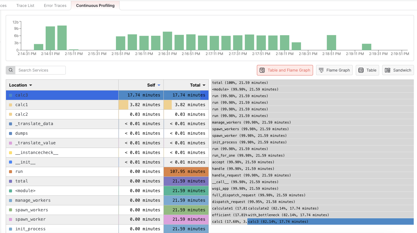
In this example, it’s clear that the `calc3` function is causing a notable bottleneck in our application.
By clicking on the function name `calc3` in the table, the function will also be highlighted in the flame graph. This will show the call stack with caller functions at the top and callee functions going toward the bottom.
# Next Steps
* [Intro to APM](https://docs.middleware.io/workflow/apm/apm-overview)
* [Databases](https://docs.middleware.io/workflow/apm/database)
* [Services](https://docs.middleware.io/workflow/apm/services)
* [APM Span List](https://docs.middleware.io/workflow/apm/span-list)
Need assistance or want to learn more about Middleware? Contact us at support\[at]middleware.io.